Aniposelib Tutorial

Aniposelib is a Python library for calibrating cameras and triangulation. Anipose uses aniposelib for the anipose calibrate and anipose triangulate, but there may be instances in which you have a DeepLabCut project and only want to use perform calibration, triangulation, and (optionally) apply 3D filters. This is a tutorial on how to use aniposelib for those who already have a DeepLabCut project.

In this tutorial, we will walk through a Python script that uses aniposelib to calibrate three cameras and triangulate the 2D detections. We will be starting from a DLC project folder that contains a model to track 20 keypoints on a hand, the same dataset that was used in the Anipose Tutorial.

Setup

If you would like to follow along as we walk through the Python code, then you may begin by downloading the following:

• The calibration and triangulation materials for the hand dataset found in this Google Drive folder. You are welcome to use any of these files as a reference at any point.
  • The Jupyter Notebook, aniposelib example.ipynb, and the Python script, aniposelib_minimal_example.py, contain the code that we will discuss in this tutorial. You may use either of these to follow along by running the code locally.
  • The three .MOV files contain the calibration videos. We used a ChArUco board to calibrate the cameras, though you also have the option of using a checkerboard.
  • The three .h5 files are from the DLC project. They encode the the most likely x and y coordinates of each keypoint on the ChArUco board. These files will be used in triangulation.
  • Optional: The aniposelib calibration file, calibration.toml, contains properties of the cameras, as well as the estimated parameter values for the camera extrinsics and intrinsics.

Installation

We will be importing modules from aniposelib, so you will need to have aniposelib installed on your machine. You can install the latest version from pip with:

pip install aniposelib

After the installation is complete, we can start the Python script by importing the necessary modules from aniposelib. More information about the aniposelib.cameras and aniposelib.boards modules can be found in the aniposelib API reference.

import numpy as np
from aniposelib.boards import CharucoBoard, Checkerboard
from aniposelib.cameras import Camera, CameraGroup
from aniposelib.utils import load_pose2d_fnames

Calibration

The following code sets some variables regarding information about the cameras and board used for calibration. The videos in vidnames correspond to the path names of the calibration videos for each of the three cameras used in calibration. The variable cam_names contains the names of the three cameras, and n_cams stores the number of cameras.

A ChArUco board was used for the calibration (this can be seen in any of the three calibration videos), so a ChArUco board object is constructed with parameters regarding information about the markers:

• X = 7 and Y = 10 because there are 7 squares in the vertical direction and 10 squares in the borizontal direction on the calibration board.
• square_length = 25 indicate that the dimensions of each square on the board is 25 mm.
• marker_length = 18.75 indicates that the dimensions of each marker within each square is 18.75 mm.
• marker_bits = 4 describes the dimension of the markers, so each marker consists of 4x4 bits.
• dict_size = 50 specifies that there are 50 types of markers in the marker dictionary.

When using aniposelib to calibrate your cameras, if you used a checkerboard for calibration, then you would construct a checkerboard object instead. More information about the ChArUco board and checkerboard objects can be found in the aniposelib API.

Lastly, cgroup is an object used to refer to all of the cameras as a single unit. When given the names of the cameras, CameraGroup.from_names() forms a CameraGroup object of the corresponding cameras. We set fisheye = true because the videos from this dataset were recorded using fisheye lens, but fisheye = false by default.

vidnames = [['calib-charuco-camA-compressed.MOV'],
            ['calib-charuco-camB-compressed.MOV'],
            ['calib-charuco-camC-compressed.MOV']]

cam_names = ['A', 'B', 'C']

n_cams = len(vidnames)

board = CharucoBoard(7, 10,
                     square_length=25, # here, in mm but any unit works
                     marker_length=18.75,
                     marker_bits=4, dict_size=50)


# the videos provided are fisheye, so we need the fisheye option
cgroup = CameraGroup.from_names(cam_names, fisheye=True)

Next, we will use the function calibrate_videos() to detect the ChArUco boards in each of the videos and calibrate the cameras accordingly. This function takes as parameters a list of lists of video filenames (one list per camera) and a calibration board object, which specifies what should be detected in the videos. Iterative bundle adjustment is used to calibrate the cameras by minimizing the reprojection error. At each iteration, this method defines a threshold for the reprojection error, then performs bundle adjustment on the points for which the reprojection error is below the determined threshold.

The code for this step will take about 15 minutes to run. Alternatively, if you don’t want to wait for the detections to be determined, you can download the calibration.toml provided in this Google Drive folder that was discussed in Setup. If you choose to do this, you can proceed to the next step, where you are shown how to load calibration.toml.

# this will take about 15 minutes (mostly due to detection)
# it will detect the charuco board in the videos,
# then calibrate the cameras based on the detections, using iterative bundle adjustment
cgroup.calibrate_videos(vidnames, board)

# if you need to save and load
# example saving and loading for later
cgroup.dump('calibration.toml')

If you saved calibration.toml to load for later or used the provided, calibration.toml file, it can be loaded with the following line of code.

## example of loading calibration from a file
## you can also load the provided file if you don't want to wait 15 minutes
cgroup = CameraGroup.load('calibration.toml')

Triangulation

During triangulation, aniposelib provides you with the option to apply 3D filters. The code shown below is an example of triangulation without filtering. First, the .h5 files are loaded with load_pose2d_fnames(), which takes a dictionary that maps the camera names to the corresponding .h5 files and a list of the camera names contained in the camera group. These .h5 files encode the the most likely 2D coordinates of each keypoint that we tracked on the hand. All of the 2D points with a score below score_threshold are removed, as they are considered erroneous.

The function triangulate() then determined the 3D coordinates of the hand given the 2D coordinates from all of the cameras. The reprojection error is then computed with reprojection_error() given the 2D coordinates associated with each keypoint from each camera and the 3D coordinates determined from all of the cameras. The reprojection error describes how well the 2D projections of a triangulated 3D point match its corresponding 2D keypoints in every camera view. Further information about the functions for triangulation and reprojection error can be found in the API.

## example triangulation without filtering, should take < 15 seconds
fname_dict = {
    'A': '2019-08-02-vid01-camA.h5',
    'B': '2019-08-02-vid01-camB.h5',
    'C': '2019-08-02-vid01-camC.h5',
}

d = load_pose2d_fnames(fname_dict, cam_names=cgroup.get_names())

score_threshold = 0.5

n_cams, n_points, n_joints, _ = d['points'].shape
points = d['points']
scores = d['scores']

bodyparts = d['bodyparts']

# remove points that are below threshold
points[scores < score_threshold] = np.nan

points_flat = points.reshape(n_cams, -1, 2)
scores_flat = scores.reshape(n_cams, -1)

p3ds_flat = cgroup.triangulate(points_flat, progress=True)
reprojerr_flat = cgroup.reprojection_error(p3ds_flat, points_flat, mean=True)

p3ds = p3ds_flat.reshape(n_points, n_joints, 3)
reprojerr = reprojerr_flat.reshape(n_points, n_joints)

Visualization

Now that we have 3D points from triangulation, we can visualize our data! We will first provide an example of how to use the output from triangulation to plot the positions of a given joint across time. The code shown below extracts and plots the x, y, and z positions of joint 0, which corresponds to the base of the hand (see Figure 1).

# plot the x, y, z coordinates of joint 0

import matplotlib.pyplot as plt
% matplotlib notebook

plt.figure(figsize=(9.4, 6))
plt.plot(p3ds[:, 0, 0])
plt.plot(p3ds[:, 0, 1])
plt.plot(p3ds[:, 0, 2])
plt.xlabel("Time (frames)")
plt.ylabel("Coordinate (mm)")
plt.title("x, y, z coordinates of {}".format(bodyparts[0]))

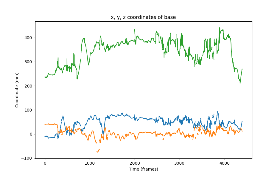
Figure 1. The x, y, and z coordinates of the joint corresponding to the base of the hand across all of the frames.

Additionally, we can visualize the position of the hand at each frame by plotting the 3D position of all of the tracked hand joints. The following code plots the 3D position of the hand determined from the the first frame in the three videos. The scheme defines which keypoints are connected in the hand, so it serves as a nice visual aid. The 3D positions of the hand are shown in Figure 2.

## plot the first frame in 3D
from mpl_toolkits.mplot3d import Axes3D
from matplotlib.pyplot import get_cmap
%matplotlib notebook

def connect(ax, points, bps, bp_dict, color):
    ixs = [bp_dict[bp] for bp in bps]
    return ax.plot(points[ixs, 0], points[ixs, 1], points[ixs, 2], color=color)

def connect_all(ax, points, scheme, bodyparts, cmap=None):
    if cmap is None:
        cmap = get_cmap('tab10')
    bp_dict = dict(zip(bodyparts, range(len(bodyparts))))
    lines = []
    for i, bps in enumerate(scheme):
        line = connect(ax, points, bps, bp_dict, color=cmap(i)[:3])
        lines.append(line)
    return lines

## scheme for the hand
scheme = [
   ["MCP1", "PIP1", "tip1"],
   ["MCP2", "PIP2", "DIP2", "tip2"],
   ["MCP3", "PIP3", "DIP3", "tip3"],
   ["MCP4", "PIP4", "DIP4", "tip4"],
   ["MCP5", "PIP5", "DIP5", "tip5"],
   ["base", "MCP1", "MCP2", "MCP3", "MCP4", "MCP5", "base"]
 ]

framenum = 0
p3d = p3ds[framenum]

fig = plt.figure(figsize=(8, 6))
ax = fig.add_subplot(111, projection='3d')
ax.scatter(p3d[:,0], p3d[:,1], p3d[:,2], c='black', s=100)
connect_all(ax, p3d, scheme, bodyparts)

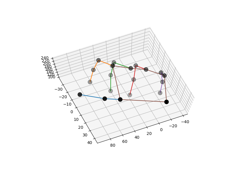
Figure 2. 3D positions of the hand joints in the first frame. These positions were determined through triangulation.